Neural Network — Implementing Backpropagation using the Chain Rule
In this post, I will go over the mathematical need and the derivation of Chain Rule in a Backpropagation process.
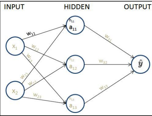
First, for this post, I will consider a really simple Neural Network architecture which is the following.
Our neural network contains one hidden layer with three nodes in it.
Every arrow in the diagram contains exactly one float value as a single weight that is adjustable. Totally there are 9 weights (6 in the first hidden layer and 3 in the second) that we need to fine-tune, so that when the input is (1,1), the output is as close to (0) as possible.
This is what we mean by training the neural network. We have not introduced a bias value yet, for simplicity purposes only — the underlying logic remains the same.
Now let's go over the basics of a Neural Network
What is a neuron
A neuron is a container that contains a mathematical function which is known as an activation function, inputs (x1 and x2 here ) , a vector of weights(w1,w2 here) and a bias(b).
A neuron first computes the weighted sum of the inputs.
The activation function is simply a mathematical function that takes in an input and produces an output.
Think of the activation function as a mathematical operation that normalizes the input and produces an output. The output is then passed forward onto the neurons on the subsequent layer.
Input layers: These layers take the independent variables as input.
Hidden (intermediate) layers: These layers connect the input and output layers while performing transformations on top of input data. Furthermore, the hidden layers contain nodes (units/circles in the above diagram) to modify their input values into higher-/lower-dimensional values. The functionality to achieve a more complex representation is achieved by using various activation functions that modify the values of the nodes of intermediate layers.
Output layer: This contains the values the input variables are expected to result in.
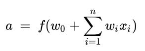
The number of nodes (circles in the preceding diagram) in the output layer depends on the task at hand and whether we are trying to predict a continuous variable or a categorical variable. If the output is a continuous variable, the output has one node. If the output is categorical with m possible classes, there will be m nodes in the output layer. Let’s zoom into one of the nodes/neurons and see what’s happening. A neuron transforms its inputs as follows:
As you can see, it is the sum of the products of weight and input pairs followed by an additional function f (the bias term + sum of products). The function f is the activation function that is used to apply non-linearity on top of this sum of products.
Calculating the hidden layer unit values
We’ll now assign weights to all of the connections. In the first step, we assign weights randomly across all the connections. And in general, neural networks are initialized with random weights before the training starts.
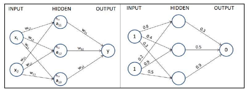
Let’s start with initial weights that are randomly initialized between 0 and 1, but note that the final weights after the training process of a neural network don’t need to be between a specific set of values. A formal representation of weights and values in the network is provided in the following diagram (left half) and the randomly initialized weights are provided in the network in the right half.
In the next step, we perform the multiplication of the input with weights to calculate the values of hidden units in the hidden layer. The hidden layer’s unit values before activation are obtained as follows:
Applying the activation function
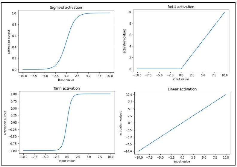
Activation functions help in modeling complex relations between the input and the output. Some of the frequently used activation functions are calculated as follows (where x is the input):
Calculating loss values
Loss values (alternatively called cost functions) are the values that we optimize for in a neural network. To understand how loss values get calculated, let’s look at two scenarios:
Categorical variable prediction
Continuous variable prediction
Calculating loss during continuous variable prediction
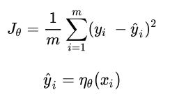
Typically, when the variable is continuous, the loss value is calculated as the mean of the square of the difference in actual values and predictions, that is, we try to minimize the mean squared error by varying the weight values associated with the neural network. The mean squared error value is calculated as follows:
Calculating loss during categorical variable prediction
When the variable to predict is discrete (that is, there are only a few categories in the variable), we typically use a categorical cross-entropy loss function. When the variable to predict has two distinct values within it, the loss function is binary cross-entropy. Binary cross-entropy is calculated as follows:
y is the actual value of the output, p is the predicted value of the output, and m is the total number of data points.
And then Categorical cross-entropy is calculated as follows:
y is the actual value of the output, p is the predicted value of the output, m is the total number of data points, and C is the total number of classes.
A simple way of visualizing cross-entropy loss is to look at the prediction matrix itself. Say you are predicting five classes — Dog, Cat, Rat, Cow, and Hen — in an image recognition problem. The neural network would necessarily have five neurons in the last layer with softmax activation. It will be thus forced to predict a probability for every class, for every data point. Say there are five images and the prediction probabilities look like so (the highlighted cell in each row corresponds to the target class):
Note that each row sums to 1. In the first row, when the target is Dog and the prediction probability is 0.88, the corresponding loss is 0.128 (which is the negative of the log of 0.88). Similarly, other losses are computed. As you can see, the loss value is less when the probability of the correct class is high. As you know, the probabilities range between 0 and 1. So, the minimum possible loss can be 0 (when the probability is 1) and the maximum loss can be infinity when the probability is 0. The final loss within a dataset is the mean of all individual losses across all rows.
Feedforward propagation — A high-level strategy of coding feedforward propagation is as follows:
Perform a sum product at each neuron.
2. Compute activation.
3. Repeat the first two steps at each neuron until the output layer.
4. Compute the loss by comparing the prediction with the actual output.
Implementing backpropagation
In feedforward propagation, we connected the input layer to the hidden layer, which then was connected to the output layer. In the first iteration, we initialized weights randomly and then calculated the loss resulting from those weight values. In backpropagation, we take the reverse approach. We start with the loss value obtained in feedforward propagation and update the weights of the network in such a way that the loss value is minimized as much as possible.
The loss value is reduced as we perform the following steps:
Note that the update made to a particular weight is proportional to the amount of loss that is reduced by changing it by a small amount. Intuitively, if changing a weight reduces the loss by a large value, then we can update the weight by a large amount. However, if the loss reduction is small by changing the weight, then we update it only by a small amount.
So how does a Neural Networks update weights and Biases during Back Propagation?
Ans is — Backpropagation reduce the error by changing the values of weights and biases. To do this during Backpropagation we calculate the rate of change of error w.r.t rate of change in weight.
Note that the update made to a particular weight is proportional to the amount of loss that is reduced by changing it by a small amount.
Intuitively this makes sense, because if changing a weight reduces the loss by a large value, then we can update the weight by a large amount. However, if the loss reduction is small by changing the weight, then we update it only by a small amount.
How Chain Rule in Back Propagation makes the calculations massively efficient?
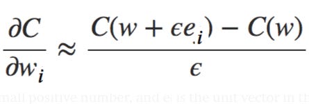
First, consider the cost as a function of the weights C=C(w) alone. You number the weights w₁,w₂,…, and want to compute ∂C/∂wᵢ for some particular weight wᵢ. An obvious way of doing that is to use the approximation
where ϵ>0 is a small positive number, and eᵢ is the unit vector in the iᵗʰ direction. In other words, we can estimate ∂C/∂wᵢ by computing the cost C for two slightly different values of wᵢ, and then applying the above equation. The same idea can be used to compute the partial derivatives ∂C/∂b with respect to the biases. But there’s a problem with this approach, which is when dealing with millions of weights this approach will be impossibly slow or sometimes can not be realistically implemented at all.
To understand why it is like so, imagine we have a million weights in our network. Then for each distinct weight wᵢ we need to compute C(w+ϵeᵢ) in order to compute ∂C/∂wᵢ. That means that to compute the gradient we need to compute the cost function a million different times, requiring a million forward passes through the network (per training example).
And that's where the chain rule in Back-propagation comes to save us, with a specific order of operations that is highly efficient.
What’s clever about backpropagation is that it enables us to simultaneously compute all the partial derivatives ∂C/∂wᵢ using just one forward pass through the network, followed by one backward pass through the network.
And so the total cost of backpropagation is roughly the same as making just two forward passes through the network. Compare that to the million and one forward passes of the previous method.
Now Finally the actual Mathematical Derivation of Chain Rule
First, take a look at our Neural Network again.
The hidden layer activation value (sigmoid activation) is calculated as follows:
Note that, this change in the loss value C with respect to the change in weight W_11 is what is THE MOST IMPORTANT thing to calculate during the Backpropagation part of Neural Network Training. And hence we need to find a way to calculate this as optimally as possible.
Note that, in the preceding equation, we have built a chain of partial differential equations in such a way that we are now able to perform partial differentiation on each of the four components individually and ultimately calculate the derivative of the loss value with respect to weight value w_11
Why exactly we are calculating this Partial Derivative applying Chain Rule
We create a chain so that each individual partial derivative can be easily calculated and we get the derivative of two variables which are not directly connected i.e. inner layer weights and the Loss
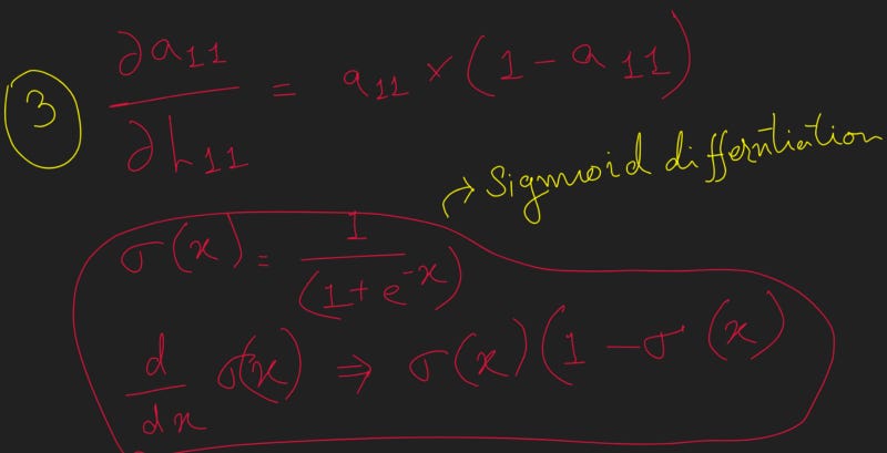
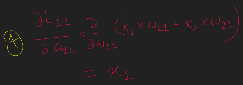
Now, the individual partial derivatives in the preceding equation are computed as follows:
Note that the preceding equation (3 ) comes from the fact that the derivative of the sigmoid function is..
So the finally, with all the above 4 component wise partial differentiation in place, the gradient of the loss value with respect to is calculated by replacing each of the partial differentiation terms with the corresponding value as calculated in the previous steps as follows:
From the preceding formula, we can see that we are now able to calculate the impact on the loss value of a small change in the weight value (the gradient of the loss with respect to weight) without brute-forcing our way by recomputing the feedforward propagation again.
And now finally, we will go ahead and update the weight value as follows:
Link to my Youtube Video explaining the entire flow.

